Nonlinear inversion of seismic waveforms
1.1 Introduction
The goal of geophysical inversion is the estimation of a set of physical parameters which best describe a postulated earth model. The estimated parameters are those which best fit a theoretical prediction (model response) to a set of observations. Inversion of seismic waveforms for rock and pore fluid elastic parameters is perhaps the most challenging inverse problem encountered in exploration geophysics. Little progress has been made towards its solution, even though great progress on seismic inversion theory and practice have been made in the last decade by numerous authors (Bamberger et al., 1982; Tarantola et al., 1982, 1984; Gray et al., 1984; Menke, 1984; Keys, 1986 and Kennett et al., 1988). Many global and local optimization algorithms developed in applied mathematics and statistics have been applied to seismic inversion. Theoretically, global optimization algorithms may be the best inverse problem solver. However, the Monte-Carlo search they employ is often computationally too expensive to realize on available computers, especially in seismic inversion, where the number of model parameters is large. In contrast, local optimization algorithms are computationally inexpensive. But the optimized model parameters will not, in general, be a unique solution to the inverse problem. Because there are a large number of model parameters involved in the seismic inverse problem, various local optimization algorithms are widely used. We use a local minimization algorithm as the inverse problem solver in our nonlinear seismic inversion technique below.
Many seismic modeling techniques have also been developed and widely used as forward models (e.g., the convolution model in travel time domain, finite difference and finite element solutions of seismic wave propagating equations, and kinematics ray-tracing). The decision of which inverse and forward algorithms to use in a particular seismic inversion is problem-dependent. However, without sufficient data to solve for a specific set of earth's parameters, the results of all inversion, however sophisticated, are meaningless. Once we determine which set of model parameters to be estimated, the forward and inverse problem solvers can then be selected for the specific seismic inversion. The forward problem determines whether the seismic inversion is linear or nonlinear (i.e., if the modeled seismic response is a linear or nonlinear function of the model parameters). The importance of the linearity/nonlinearity distinction stems from the inversion algorithms. Only linear problems have an exact solution. Local optimization algorithms work by treating a nonlinear problem as a linear one. This linearization involves the computation of the gradient of the predicted data with respect to the model parameters.
Two types of gradients (linear and nonlinear), are widely used in the inversion of seismic waveforms. The choice depends on the nature of the seismic forward model. Because most geophysical observations are nonlinearly correlated to the earth's physical parameters, nonlinear gradients are preferred, even when the nonlinearity is only extended to the second order.
Given horizontally stacked and migrated 3-D seismic data, each seismic trace in the seismic volume can be treated as a zero-offset seismic trace. Acoustic impedance, rather than propagation velocity, is the appropriate model parameter, since the zero-offset seismic trace is only sensitive to the former.
In this chapter, we present a one-dimensional nonlinear inversion technique that can be used to invert vertical seismic traces to obtain acoustic impedance as a function of two-way travel time. The technique uses a convolution forward model to compute the seismic trace from the acoustic impedance function. A modified Levenberg-Marquardt minimization algorithm (More, 1977) is implemented to solve the nonlinear inverse problem. The formulation of the one-dimensional, nonlinear inversion include the imposition of constraints onto the objective function using covariance functions. Our nonlinear seismic inversion uses several zero-phase seismic source functions, that are constructed by using digital filter design (approximated by Ricker wavelets) and that extract autocorrelation functions (Robinson et al., 1980). The estimated acoustic functions derived from both synthetic seismic traces and real seismic traces using different implementation techniques are also presented. By using these approaches, the frequency bandwidth of estimated acoustic impedance functions can be forced to be the same as that of input seismic traces. The results obtained from numerical experiments on the synthetic and real seismic traces also suggest that the modified Levenberg-Marquardt algorithm is as robust an approximation of the impedance function as can be obtained when appropriate constraints are present.
1.2 Convolution seismic forward model
In laterally homogeneous acoustic media, seismic propagation can be approximately modeled by the convolution of two time series
![]() ,
(1.1)
,
(1.1)
where
![]() is the seismic trace (acoustic pressure) as a function of travel time,
is the seismic trace (acoustic pressure) as a function of travel time,
![]() is the seismic source function, and
is the seismic source function, and
![]() is the reflection coefficient series. The interbedded multiples are not
considered in this equation. In discrete form,
is the reflection coefficient series. The interbedded multiples are not
considered in this equation. In discrete form,
![]() is given by
is given by
![]() ,
(1.2)
,
(1.2)
where
![]() is the reflection coefficient of i-th interface,
is the reflection coefficient of i-th interface,
![]() is the acoustic impedance, which is the product of wave propagation velocity
times bulk density. i and i+1 are the indices representing the layer number
above and below the i-th interface. Given a known seismic source function
is the acoustic impedance, which is the product of wave propagation velocity
times bulk density. i and i+1 are the indices representing the layer number
above and below the i-th interface. Given a known seismic source function
![]() and acoustic impedance function
and acoustic impedance function
![]() ,
the seismic response of the media can be generated by the convolution model
defined by Eq. 1.1.
,
the seismic response of the media can be generated by the convolution model
defined by Eq. 1.1.
The seismic source function
![]() in seismic inversion is typically unknown. In practice, due to the
band-limited nature of seismic observations, seismic source functions or
wavelets are approximated by bandpass filters whose frequency ranges are at
least as broad as that of the observed seismic data. Such filters are usually
designed in the frequency domain, and the inverse Fourier transform of these
frequency filters can be used as seismic source functions. In our experiments,
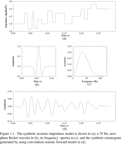
the seismic response of a synthetic layer model is the convolution of a
zero-phase Ricker wavelet (peak frequency of 35 Hz) with a reflectivity
function derived from the acoustic impedance function. The acoustic impedance
model, synthetic seismogram and the seismic source function are shown in
(Figure 1.1). This synthetic seismic trace is used as the example in numerical
experiments to test the proposed nonlinear seismic inversion technique
described later in this chapter.
in seismic inversion is typically unknown. In practice, due to the
band-limited nature of seismic observations, seismic source functions or
wavelets are approximated by bandpass filters whose frequency ranges are at
least as broad as that of the observed seismic data. Such filters are usually
designed in the frequency domain, and the inverse Fourier transform of these
frequency filters can be used as seismic source functions. In our experiments,
the seismic response of a synthetic layer model is the convolution of a
zero-phase Ricker wavelet (peak frequency of 35 Hz) with a reflectivity
function derived from the acoustic impedance function. The acoustic impedance
model, synthetic seismogram and the seismic source function are shown in
(Figure 1.1). This synthetic seismic trace is used as the example in numerical
experiments to test the proposed nonlinear seismic inversion technique
described later in this chapter.
1.3 Nonlinear inversion of seismic waveforms
Acoustic pressure variations observed on the earth's surface produced by a seismic source are nonlinearly correlated with the earth's acoustic parameters. The acoustic impedance can be nonlinearly estimated from these seismic measurements made at the earth's surface. Acoustic impedance is found by minimizing the least-squares error between the observed and predicted acoustic pressures (seismic traces). In reviewing the numerous minimization algorithms developed to solve least-squares problems, we have found that the large-scale nonlinear minimization problem can be efficiently solved on modern workstations by using a modified version of a rather classical algorithm, the Levenberg-Marquardt method (Levenberg, 1944; Marquardt, 1963; Keys, 1986 and Lines et al., 1984).
1.3.1 Formulation of the nonlinear seismic inversion
The seismic inversion can be formulated as an optimization problem of the
form: find a set of model parameters
![]() which minimizes an objective function F(m):
which minimizes an objective function F(m):
![]() .
(1.3)
.
(1.3)
Here
![]() is a vector representing samples of the observed seismic trace,
is a vector representing samples of the observed seismic trace,
![]() contains samples of the modeled seismic trace,
contains samples of the modeled seismic trace,
![]() are model parameters (acoustic impedance, source wavelet parameters),
are model parameters (acoustic impedance, source wavelet parameters),
![]() is an a priori model independently estimated from other data source, and
is an a priori model independently estimated from other data source, and
![]() denotes a weighted L2-norm. This norm employs covariance functions
denotes a weighted L2-norm. This norm employs covariance functions
![]() and
and
![]() (Tarantola, 1984) such that the first and second terms on right-hand side in
Eq. 1.3 can be further expanded as:
(Tarantola, 1984) such that the first and second terms on right-hand side in
Eq. 1.3 can be further expanded as:
![]() (1.4)
(1.4)
and
![]() ,
(1.5)
,
(1.5)
respectively.
The estimation of the covariance functions, namely,
![]() and
and
![]() ,
are of great importance in nonlinear seismic inversion because they quantify
uncertainties in data space and model space. Through covariance functions, we
are able to impose the a priori set of model parameters to constrain the
inversion process. These functions can be chosen so that the estimated model
parameters are smooth. They also implies that the a posteriori
variance of each model parameter is centered at the corresponding samples
of the a priori model. Unbounded oscillations in the solutions are
prevented by constraints applied in this way, and the estimated model is
constrained to have a certain degree of resemblance to the a priori
model. When the a priori model is set to the low-frequency trend of
the acoustic impedance function, the degree of nonuniqueness in the estimated
impedance function is often dramatically reduced. The uncertainties of
estimated model parameters can also be quantified by means of using row vectors
of the covariance function predetermined in model space. Construction for the
covariance functions are discussed in detail in specific numerical experiments
later in this chapter.
,
are of great importance in nonlinear seismic inversion because they quantify
uncertainties in data space and model space. Through covariance functions, we
are able to impose the a priori set of model parameters to constrain the
inversion process. These functions can be chosen so that the estimated model
parameters are smooth. They also implies that the a posteriori
variance of each model parameter is centered at the corresponding samples
of the a priori model. Unbounded oscillations in the solutions are
prevented by constraints applied in this way, and the estimated model is
constrained to have a certain degree of resemblance to the a priori
model. When the a priori model is set to the low-frequency trend of
the acoustic impedance function, the degree of nonuniqueness in the estimated
impedance function is often dramatically reduced. The uncertainties of
estimated model parameters can also be quantified by means of using row vectors
of the covariance function predetermined in model space. Construction for the
covariance functions are discussed in detail in specific numerical experiments
later in this chapter.
1.3.2 Implementation of the modified Levenberg-Marquardt algorithm
A modified Levenberg-Marquardt gradient algorithm developed by More (1977) is used to solve our inverse problem. The classical Levenberg-Marquardt algorithm is a linear minimization algorithm that uses only the linear gradient of modeled response with respect to model parameters. It minimizes the objective function in the form of Eq. 1.3 in an iterative manner. More importantly, a large number of model parameters can be solved for without heavy computational burden. In searching for the new model parameters, the algorithm intrinsically imposes a finite quantity to the variation of the updating steps (Levenberg, 1944 and Marquardt, 1963) so that the next step taken is not allowed to change too much from the previous step. The method distinguishes itself from other gradient methods by combining the nonlinear least-squares method and steepest descent method to choose each updating step of model parameters. By adjusting the Lagrange multiplier, the Levenberg-Marquardt approach selects either the least-squares method or the steepest descent method to dominate the parameter search. If the computed gradients are small, the steepest descent method can be used to effectively speed up the global convergence by adding a significant constant to the diagonal entities of the gradient matrix. When the objective functions are getting less significant, , the least-squares method can be used to seek the global convergence by adding a constant less than unity to the diagonal entities of the gradient matrix. In addition, the convergence rate of the Levenberg-Marquardt method is also increased by using an intrinsic scaling factor. The modification made to the Levenberg-Marquardt method by More (1977) relies on incorporating the second derivative of gradients of the objective function versus model parameters, i.e., the Hessian matrix, into estimating model parameters. The added quadrature form in gradient space makes the modified Levenberg-Marquardt method essentially a nonlinear minimization method with global convergence characteristics. These are the reasons that the modeled seismic traces match the observed seismic traces almost perfectly in our numerical experiments presented later. The seismic inverse problems, whose objective functions are nonlinear functions of model parameters can be better resolved by using this modified nonlinear method than by using the original Levenberg-Marquardt method. The proper use of the implicitly scaled variables and an optimal choice for the correction are the main advantages over other gradient methods. The use of the implicitly scaled variables achieves scale invariance, and limits the size of the updating steps in directions where the objective functions are changing rapidly. The optimal choice of the updating steps guarantees global convergence from starting model parameters that are far from the solution and a fast rate of convergence for problems with small residuals.
Starting from a set of initial model parameters, the seismic forward problem
is first solved by using the convolution method (Eq. 1.1) and a known seismic
source function to predict the seismic response. Using the predetermined
covariance functions in model space and data space, the objective function, or
misfit function, can then be computed (Eq. 1.3). By perturbing each model
parameters by an amount
![]() ,
we can compute the gradient matrix (Jacobian matrix) of the objective function
with respect to each model parameter using a forward difference approximation
of the form
,
we can compute the gradient matrix (Jacobian matrix) of the objective function
with respect to each model parameter using a forward difference approximation
of the form
![]() .
(1.6)
.
(1.6)
Here
![]() is a small perturbation in the j-th model parameter.
is a small perturbation in the j-th model parameter.
![]() and
and
![]() are the function evaluated at the current model
are the function evaluated at the current model
![]() and the function evaluated at the model
and the function evaluated at the model
![]() with the perturbation of
with the perturbation of
![]() added to its j-th component. The Jacobian matrix provides the gradients
necessary for the modified Levenberg-Marquardt algorithm to iteratively define
the model parameters until the "stopping" criteria are satisfied. For its
simplicity and convenience for adding extra model parameters to the inversion,
we use the forward difference approximation to compute the gradient matrix. It
is also possible to derive the analytic gradients using the chain rule to
compute Jacobian matrix in our case.
added to its j-th component. The Jacobian matrix provides the gradients
necessary for the modified Levenberg-Marquardt algorithm to iteratively define
the model parameters until the "stopping" criteria are satisfied. For its
simplicity and convenience for adding extra model parameters to the inversion,
we use the forward difference approximation to compute the gradient matrix. It
is also possible to derive the analytic gradients using the chain rule to
compute Jacobian matrix in our case.
At each iteration, the current model and its Jacobian matrix are used to an update set of model parameters that reduce the current objective function. The sum of squared errors between the model response and the observations are expected to be continuously reduced. Two convergence tests are implemented in the algorithm to terminate the iterative search for the minimal objective function:
1) The relative changes in the objective function between consecutive iterations becomes less than the preset tolerance.
2) The objective function has reached the tolerance that is set to the machine precision.
When these convergence criteria have been satisfied, the estimated model parameters have created a model which has matched the data within our specifications.
1.4 Numerical experiments
Many factors can adversely affect the seismic inversion. When the data contain noise, the observed seismic data cannot be perfectly predicted by theory. No possible model exactly predicts the model parameters. We use a synthetic and a real seismic trace extracted from a 3-D seismic survey at a well location to examine the feasibility of the proposed nonlinear seismic inversion method. The inversion of the seismograms is carried out according to both known and unknown conditions of seismic source functions, reflection interfaces, and acoustic impedance constraints. The inversion results are compared to the true impedance model or to the impedance log. The latter is derived from sonic velocity and bulk density logs measured in the well.
1.4.1 Inversion of the synthetic seismic data
Different approaches can be used to invert the synthetic seismic trace (Figure 1.1) (d) for acoustic impedance depending upon which parameters are assumed to be known.
The synthetic seismogram (Figure 1.1) (d) consists of 286 discrete points. This observed data is always expressed as the vector:
 .
(1.7)
.
(1.7)
Although the modified Levenberg-Marquardt algorithm used in this thesis can
handle underdetermined problems (the number of parameters, n, to be solved for
is greater than the number of data observations, m), we have chosen to use
either an even or overdetermined algorithm (the number of unknown parameters is
less or equal to the number of observations). Because the seismic inverse
problem is underdetermined in a general sense, the observations made in
reflection seismic experiments are always fewer than those required to solve
for rock and pore fluid acoustic or elastic parameters. Whether the full scale
impedance model
![]() or the parametric impedance model
or the parametric impedance model
![]() should be used depends upon whether a priori knowledge of the reference
source function
should be used depends upon whether a priori knowledge of the reference
source function
![]() ,
reference impedance model
,
reference impedance model
![]() ,
and their covariances are known. Numerical examples describing different
approaches to invert the synthetic seismic trace are presented in the following
cases.
,
and their covariances are known. Numerical examples describing different
approaches to invert the synthetic seismic trace are presented in the following
cases.
1.4.2 Unconstrained parametric nonlinear inversion
We first investigate the overdetermined case with nz=18 and nw=133 (nz is the number of samples in acoustic impedance function and nw is the number of samples in the wavelet function). The seismic source function as well as the acoustic impedance function are considered unknown.
A 30 Hz, zero-phase wavelet (nw=133) is used as the initial source function. The number of reflection interfaces, nz, and the locations of reflection interfaces are known, then we can form the model parameter vector:
![]() ,
(1.8)
,
(1.8)
where
![]() and
and
![]() are column vectors of the source and impedance functions. For unconstrained
nonlinear inversion, the objective function is simply given by
are column vectors of the source and impedance functions. For unconstrained
nonlinear inversion, the objective function is simply given by
 ,
(1.9)
,
(1.9)
where
![]() and
and
![]() are components of the observed and modeled seismic traces. We take the initial
acoustic impedance function to be the linearly-regressed trend of the true
impedance function. The seismic source function, and modeled seismic trace
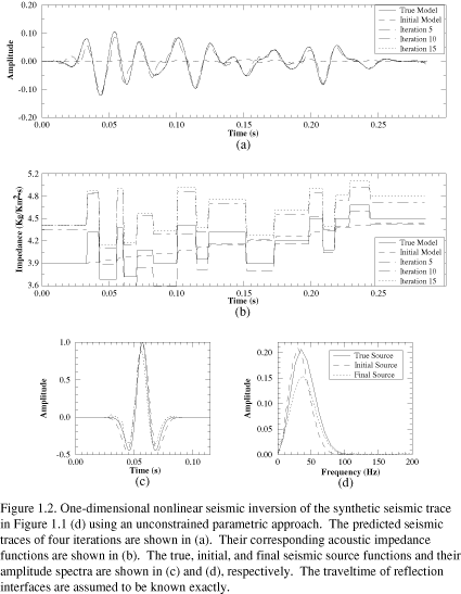
estimated at four iterations are computed and shown in (Figure 1.2). The modeled
seismic trace at final iteration (15th iteration) almost exactly fits the
synthetic seismic trace (Figure 1.2) (a). The final, estimated impedance
function departs from the true model a great deal (Figure 1.2) (b), but the
relative changes in acoustic impedance are reproduced. The relative error (the
average of the relative errors at all samples) between the estimated and the
actual impedance functions is 10.1%. The shape of source function at the final
iteration matches the true seismic source function except for some
perturbations at the beginning and the end of the source function
(Figure 1.2) (c). The amplitudes of the estimated source function are slightly smaller
than those of the true seismic source function. The enlargement of the
estimated acoustic impedance function is found to be proportional to the
decreasing magnitude of the estimated source function. Frequency spectra of
the initial, estimated, and true seismic source functions are shown in
(Figure 1.2) (d). The frequency range of the true seismic source function is
well-resolved by the estimated source function.
are components of the observed and modeled seismic traces. We take the initial
acoustic impedance function to be the linearly-regressed trend of the true
impedance function. The seismic source function, and modeled seismic trace
estimated at four iterations are computed and shown in (Figure 1.2). The modeled
seismic trace at final iteration (15th iteration) almost exactly fits the
synthetic seismic trace (Figure 1.2) (a). The final, estimated impedance
function departs from the true model a great deal (Figure 1.2) (b), but the
relative changes in acoustic impedance are reproduced. The relative error (the
average of the relative errors at all samples) between the estimated and the
actual impedance functions is 10.1%. The shape of source function at the final
iteration matches the true seismic source function except for some
perturbations at the beginning and the end of the source function
(Figure 1.2) (c). The amplitudes of the estimated source function are slightly smaller
than those of the true seismic source function. The enlargement of the
estimated acoustic impedance function is found to be proportional to the
decreasing magnitude of the estimated source function. Frequency spectra of
the initial, estimated, and true seismic source functions are shown in
(Figure 1.2) (d). The frequency range of the true seismic source function is
well-resolved by the estimated source function.
1.4.3 Constrained parametric nonlinear inversion
We impose physical constraints on the inversion through the choice of
![]() and
and
![]() (Eq. 1.5). The true acoustic impedance function is treated as a random
variable, estimated with respect to an a priori impedance model
independently obtained from other geophysical experiments. In addition,
uncertainty of the observed seismic data can also be estimated to account for
noise contamination. We use a narrow Gaussian distribution function as the
a priori and a posteriori distribution in both data and model space.
The covariance functions, Cd and Cm,
represents a priori information on the smoothness of the data and model
parameters. They are of the matrix forms (Tarantola, 1984):
(Eq. 1.5). The true acoustic impedance function is treated as a random
variable, estimated with respect to an a priori impedance model
independently obtained from other geophysical experiments. In addition,
uncertainty of the observed seismic data can also be estimated to account for
noise contamination. We use a narrow Gaussian distribution function as the
a priori and a posteriori distribution in both data and model space.
The covariance functions, Cd and Cm,
represents a priori information on the smoothness of the data and model
parameters. They are of the matrix forms (Tarantola, 1984):
![]() (1.10)
(1.10)
and
![]() ,
(1.11)
,
(1.11)
respectively. Where in Eq. 1.10,
![]() is the postulated maximal variance of the i-th component of the observed
seismic data.
is the postulated maximal variance of the i-th component of the observed
seismic data.
![]() is the correlation length and t is time. The index, k, is a relative index, of
which the components of
is the correlation length and t is time. The index, k, is a relative index, of
which the components of
![]() are non-zero only when
are non-zero only when
![]() .
.
The two element matrices in Eq. 1.11,
![]() and
and
![]() ,
can also be analytically estimated using the same form of Eq. 1.10. They are
covariance functions of seismic source function and impedance function given by
(Tarantola, 1984):
,
can also be analytically estimated using the same form of Eq. 1.10. They are
covariance functions of seismic source function and impedance function given by
(Tarantola, 1984):
![]() (1.12)
(1.12)
and
![]() ,
(1.13)
,
(1.13)
respectively. Here ,
![]() ,
and
,
and
![]() are the postulated maximal variances of i-th component of the model parameter
function, consisting of the source function and acoustic impedance function.
are the postulated maximal variances of i-th component of the model parameter
function, consisting of the source function and acoustic impedance function.
The diagonal elements of these covariance matrices are measures of the
distribution width in data or model space. The off-diagonal elements indicate
the degree to which pairs of data or model parameters are correlated (Menke,
1984). For a uncorrelated random variable, only the diagonal elements are
none-zero. The covariance function constructed in this way is a symmetric,
banded matrix, only elements along the main diagonal are none zero, and the
diagonal elements are of the maximal variances. The width of each column
vector (the number of non-zero elements) in
![]() is the measure of uncertainty of each observed sample and the relationship to
its neighboring samples.
is the measure of uncertainty of each observed sample and the relationship to
its neighboring samples.
As in the previous experiments, an a priori impedance model
![]() (nz=18) is obtained from fitting a linear trend to the true
impedance. The reference impedance and the initial impedance is taken to be
equal to the true impedance, too. The covariance function of impedance
(nz=18) is obtained from fitting a linear trend to the true
impedance. The reference impedance and the initial impedance is taken to be
equal to the true impedance, too. The covariance function of impedance
![]() is computed according to Eq. 1.13, and variance size is set to 20% of the
reference impedance function at each interface. The initial seismic source
function is again assumed to be a 30 Hz, zero-phase Ricker wavelet
(nw=131). And the reference source function
is computed according to Eq. 1.13, and variance size is set to 20% of the
reference impedance function at each interface. The initial seismic source
function is again assumed to be a 30 Hz, zero-phase Ricker wavelet
(nw=131). And the reference source function
![]() is assumed to be a 40 Hz zero-phase wavelet of the same length. The covariance
function
is assumed to be a 40 Hz zero-phase wavelet of the same length. The covariance
function
![]() is computed according to Eq. 1.12, and the variance size is set to that of the
initial source function. The covariance function
is computed according to Eq. 1.12, and the variance size is set to that of the
initial source function. The covariance function
![]() is computed using the variance of the seismic trace. Since we do not have a
way of measuring the level of noise contamination in the observed seismic
trace, the variance of the seismic trace is set to be a fraction (1%) of the
maximum seismic amplitude.
is computed using the variance of the seismic trace. Since we do not have a
way of measuring the level of noise contamination in the observed seismic
trace, the variance of the seismic trace is set to be a fraction (1%) of the
maximum seismic amplitude.
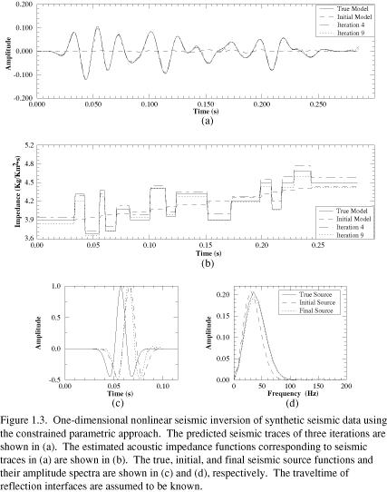
Because the objective function (Eq. 1.3) is the sum of two terms having different sizes, we scale one relative to the other so that the inversion is not dominated by either of them. The estimated acoustic impedance functions, predicted seismic traces, and seismic source functions are shown in (Figure 1.3). Both estimated impedance and seismic source functions are better resolved than in the unconstrained inversion. The average relative error between the estimated acoustic impedance function and the true impedance function is 1.5%. The imperfect match between the estimated and true impedance may be caused by improper choice of the covariance functions, the large departure of the reference model from the true model, or the improper scaling factors applied to different data types. Repeated experiments with minor modification on the a priori model (including both seismic source function and impedance model) give similar results, suggesting that this is the limit of precision of this inversion method. The optimized seismic source function is well-resolved regardless of the differences in the starting source function.
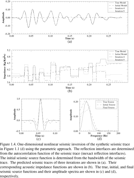
We have found that the location of the exact reflection interfaces are difficult to obtain directly through inversion. We therefore use a pre-processing step that estimates reflector depth directly from the data. The observed seismic trace is cross-correlated with the a priori seismic source function. Peaks and troughs of the cross-correlation function are assumed to indicate the depths of reflection interfaces. Results from the test inversion, using the same covariance functions from the last example, are not as accurate as before. The relative error of the estimated acoustic impedance function is 4.7% (Figure 1.4) (b), which is about half of that obtained from the unconstrained inversion (Figure 1.2) (b). There are a total of twenty-two interfaces are detected, more than that of the true model, yet a few key interfaces are missing. Although the predicted seismic trace is as good as those from the previous two experiments, the source function is poorer, being less symmetric in shape. The frequency content of the estimated seismic source function is also different from the true source function (Figure 1.4) (c).
1.4.4 Constrained nonlinear full-scale inversion
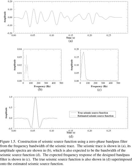
Given the synthetic seismogram in (Figure 1.1) (d), its seismic source function is designed to be zero-phase and to have the same frequency bandwidth as the seismic trace (Figure 1.5) (a) and (b). A trapezoidal function is fit to the spectra of the seismic trace, and a zero-phase source function is built from it using an inverse Fourier transform (Figure 1.5) (c). The principal lobes of the two functions are nearly identical, although some differences are observed on the sidelobes (Figure 1.5) (d).
In the full-scale inversion process, the model parameter vector
![]() contains only impedances, sampled as finely as the seismic trace:
contains only impedances, sampled as finely as the seismic trace:
 .
(1.14)
.
(1.14)
We use the same choices for the covariance functions,
![]() ,
and
,
and
![]() as before. The estimated impedance function and modeled seismic trace are
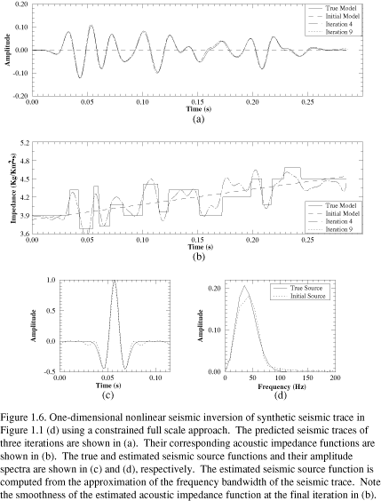
shown in (Figure 1.6). As expected, the errors between the observed and modeled
seismic traces are small (Figure 1.6) (a). The estimated impedance function
varies smoothly with depth, an effect due to the particular choice of
as before. The estimated impedance function and modeled seismic trace are
shown in (Figure 1.6). As expected, the errors between the observed and modeled
seismic traces are small (Figure 1.6) (a). The estimated impedance function
varies smoothly with depth, an effect due to the particular choice of
![]() .
No distinct layers are recovered. Nevertheless, the major features in the
estimated acoustic impedance function are well-resolved (Figure 1.6) (b). Two
layers between 0.152 and 0.2 seconds show oscillatory features, and are also
shifted towards large impedance values. These oscillations occur because these
layers are usually thick. The shift is caused by large departures of the
actual impedance model from the regressed trend model, which is used as the
reference model. The seismic source function used in this experiment and its
frequency spectrum are shown in (Figure 1.6) (c) and (d). The relative error of
the estimated acoustic impedance functions is 2.6%.
.
No distinct layers are recovered. Nevertheless, the major features in the
estimated acoustic impedance function are well-resolved (Figure 1.6) (b). Two
layers between 0.152 and 0.2 seconds show oscillatory features, and are also
shifted towards large impedance values. These oscillations occur because these
layers are usually thick. The shift is caused by large departures of the
actual impedance model from the regressed trend model, which is used as the
reference model. The seismic source function used in this experiment and its
frequency spectrum are shown in (Figure 1.6) (c) and (d). The relative error of
the estimated acoustic impedance functions is 2.6%.
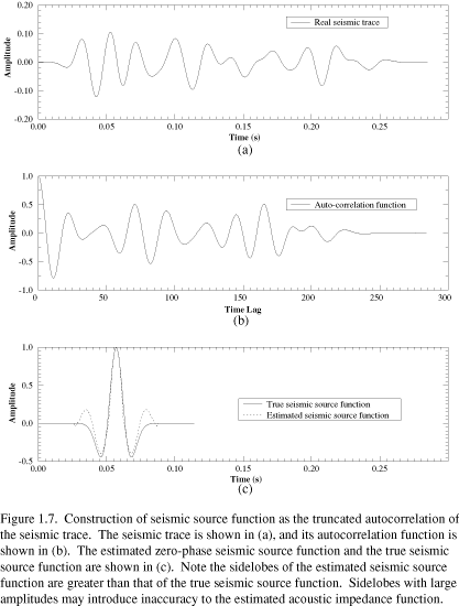
The second approach to estimating the source wavelet is to construct it from the truncated autocorrelation function of the observed seismic trace. This wavelet is symmetric and zero-phase. When the real seismic source function is minimum or mixed phase, a shaping filter is applied to adjust the phase of the estimated source function. In the following example, the zero-phase source function is used. The construction and comparison of such seismic source functions are shown in (Figure 1.7). Note that the differences between the principal peaks in the autocorrelation function and the true seismic source function are not significant (Figure 1.7) (a) and (b). However, the sidelobes of the autocorrelation function are greater than that of the true source function. Using the estimated source function that is directly constructed from the autocorrelation function may cause the estimated impedance function to be underestimated. To avoid these underestimation, sidelobes of the actual source function are scaled to about half of their original magnitude (Figure 1.7) (c).
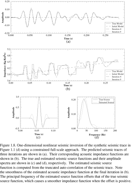
Using the new source function and with the rest of the parameter settings kept the same as the last experiment, the estimated source acoustic impedance functions and predicted seismic traces are shown in (Figure 1.8). The estimated acoustic impedance functions are similar in general to the results obtained from the trapezoidal source spectrum method (compare (Figure 1.6) (b) with (Figure 1.8) (b). Differences in the impedance functions are observed in thick layers topped at 0.16 second and 0.24 seconds. These are caused by the differences in the source functions. A thin layer between 0.012 and 0.015 seconds is resolved with underestimated impedance values just as in the previous experiment (Figure 1.6) (b) and (Figure 1.8) (b). The average relative error in the estimated acoustic impedance is also 2.6%. The frequency bandwidth of the two impedance functions is almost identical.
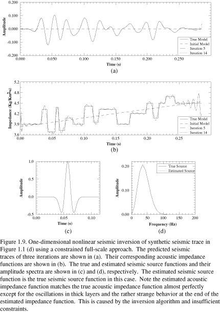
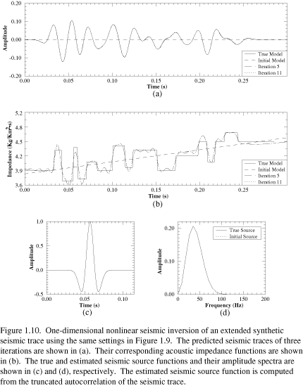
The importance of an accurate estimate of seismic source function is demonstrated in the next experiment. A 30 Hz, zero-phase Ricker wavelet is used as the estimated seismic source function (the true source function is a 35 Hz, zero-phase Ricker wavelet). The a priori impedance model is used as both reference and initial impedance. The estimated acoustic impedance function and predicted seismic traces are shown in (Figure 1.9). The estimated impedance function matches nearly all features of the true impedance model (Figure 1.9) (b). Compared to two previous experiments, the estimated impedance function is much better-resolved than the previous examples (Figure 1.6) (b), (Figure 1.8) (b), and (Figure 1.9) (b). However, low magnitude, high frequency oscillations appeared in thick layers. Despite these effects, the relative error of the estimated acoustic impedance function is 1.3%, which is less than the error obtained from the parametric inversion using the exact interface information. The largest magnitude oscillations are observed at the bottom of the estimated impedance function. They can be avoided by extending the length of seismic traces at least a wavelength. The estimated impedance function is then truncated to the length of original seismic traces (Figure 1.10). The erratic tail oscillation disappears, and the truncated acoustic impedance function is in good agreement with the true impedance model (Figure 1.10) (b). However, the oscillations still occur in the thickest layers.
1.4.5 Summary of inverting synthetic seismic data
The unconstrained nonlinear inversion is not capable of recovering the true impedance function. It can be used only to derive relative changes in true impedance function. More than one type of model parameters can be simultaneously optimized when properly constrained in the parametric seismic inversion. When exact reflection interfaces are available, the parametric technique is excellent for estimating the seismic source function. However, the estimated impedance functions are generally inaccurate when inexact reflection interfaces are used. The main disadvantage of the parametric technique is its requirement for exact interface information, thus it has limited use in inverting real seismic data. The constrained full-scale nonlinear inversion technique is the most robust method for estimating acoustic impedance from real seismic data.
1.4.6 Inversion of real seismic data
Nonlinear inversion of real seismic data is a tedious process. Imperfections of spectral division, demultiplication and deconvolution, poor amplitude preservation, migration with uncertain velocities, absence of high- and low-frequency information on seismic traces, noise, and non-vertical planar reflections can introduce tremendous difficulties. With modern seismic processing technologies, these interferences are dramatically reduced but still exist. Impedance logs measured in wells are required to constrain the inversion of such imperfect data. Better estimates of covariance functions are needed to quantify errors between estimated and measured impedance functions.
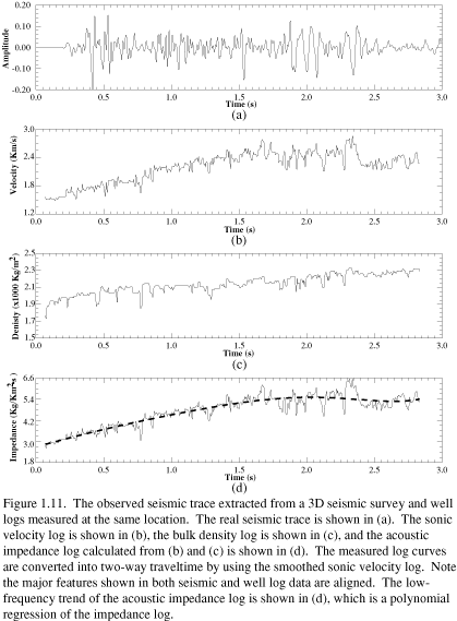
A seismic trace extracted from a 3-D stacked and migrated seismic survey in the EI-330 Field of offshore Louisiana is shown in (Figure 1.11) (a). Sonic and density logs from a well at the same location are shown in (Figure 1.11) (b) and (c). The impedance log derived from the sonic and density logs is shown in (Figure 1.11) (d).
Acoustic properties of sedimentary rocks measured by logging in wells provide
direct reference models for nonlinear seismic inversions. The low-frequency
trend regressed from impedance logs can compensate for the low-frequency
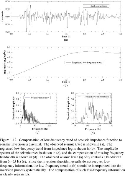
information missing in the real seismic trace (Figure 1.12) (c) and
(d). The
actual compensation is done by taking the low-frequency trend as the a
priori impedance,
![]() .
High-frequencies that are missing from the seismic traces can often be
recovered from the inversion, but the accuracy of such estimates is often
questionable. Within these limits, the broader the bandwidth of estimated
impedance, the more readily it can be applied to real earth reservoir
characterization and other geological tasks.
.
High-frequencies that are missing from the seismic traces can often be
recovered from the inversion, but the accuracy of such estimates is often
questionable. Within these limits, the broader the bandwidth of estimated
impedance, the more readily it can be applied to real earth reservoir
characterization and other geological tasks.
Similar to the inverse problem formulated for the synthetic seismic data, the observed seismic trace is the data (n samples), and the model to be estimated contains only impedance components (m samples). We use our constrained, full-scale, nonlinear seismic inversion to estimate the acoustic impedance function, thus, it is an even determined problem (here n=m).
Because we use a convolution model to predict the seismic response (Eq. 1.1), the interferences mentioned above are not considered. While the post-stack seismic data do contain noise and multiple reflection contamination, we must consider the possibility that the post-stack seismic data has uncertainties of being accurate. If we assume noise contamination in the observed seismic trace is random with a Gaussian distribution, we can again write the covariance function of data space as
![]() (i=0, n-1, n=751), (1.15)
(i=0, n-1, n=751), (1.15)
where
![]() is the postulated variance size of i-th sample of the seismic trace, which is
set to 10% of the absolute maximum amplitude in the trace. To impose the
low-frequency constraints, the covariance function of model space is estimated
by
is the postulated variance size of i-th sample of the seismic trace, which is
set to 10% of the absolute maximum amplitude in the trace. To impose the
low-frequency constraints, the covariance function of model space is estimated
by
![]() ,
(i=0, m-1, m=751), (1.16)
,
(i=0, m-1, m=751), (1.16)
where
![]() is the postulated variance size of the i-th sample of the impedance function.
is the postulated variance size of the i-th sample of the impedance function.
![]() is the correlation length within which the impedance is expected to be smooth.
Because seismic resolution is lower than that of the impedance log,
is the correlation length within which the impedance is expected to be smooth.
Because seismic resolution is lower than that of the impedance log,
![]() is set to 28 ms in length (7 samples of 4 ms sampling rate).
is set to 28 ms in length (7 samples of 4 ms sampling rate).
![]() is set to 20% of the impedance value at the i-th sample of the a priori
impedance model
is set to 20% of the impedance value at the i-th sample of the a priori
impedance model
![]() .
.
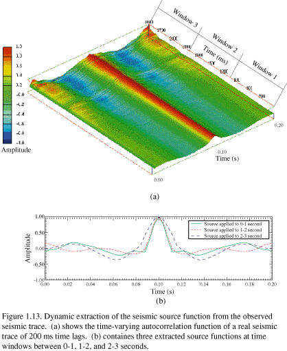
Extraction of the seismic source function from real seismic data requires special attention. Geological formations are low-pass filters to seismic waves. High frequencies are lost as waves propagate deep into the earth's crust. Normally, the stacked and migrated seismic traces are filtered differently along their length to account for the lower and lower frequency content. Bandpass filters with different frequency bandwidths are used in different time windows. (Figure 1.13) (a) illustrates the different frequency bandwidths that were applied to the seismic trace shown in (Figure 1.11) (a). The autocorrelation function at each time step is computed from a truncated seismic trace segment that starts from the current time and contains 251 subsequent sample points of the seismic trace. Three different seismic filters apparently have been applied to filter the seismic trace within windows 0-1, 1-2, and 2-3 seconds, respectively. Three extracted zero-phase seismic source functions for these three windows are shown in (Figure 1.13) (b). The frequency bandwidth of these extracted source function decreases from shallow to deep. These three different seismic source functions are used in the convolution model, constraining, the predicted seismic trace to have the same frequency content as the observed seismic trace.
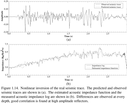
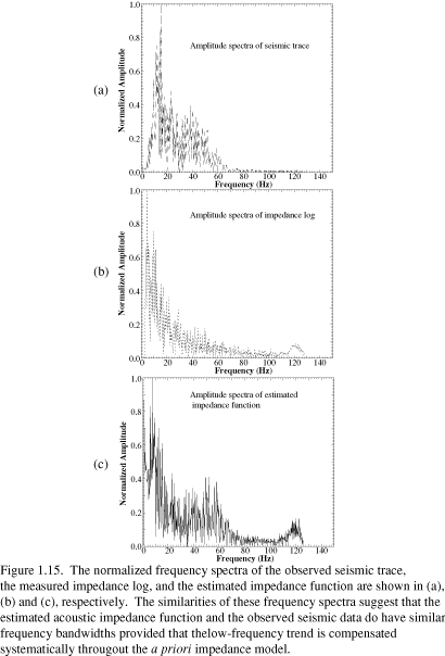
The estimated impedance function and predicted seismic trace are shown in (Figure 1.14). The predicted seismic trace matches the observed seismic trace well even though the estimated seismic source functions are not necessarily the true seismic source functions. The relative error of the estimated impedance function is 22.5%. However, the match is particularly good at times where significant seismic amplitude contrasts exist. For example, the average relative error between 1.7 and 2.5 seconds is only about 5.7%, within which more than five major hydrocarbon reservoirs are present. The large differences between the observed and estimated impedance functions may be attributed to differences in measuring techniques and frequency range (10 KHz for sonic logging, 30 Hz for the seismic profiling), because the acoustic properties measured at sonic logging frequency are strongly affected by intrinsic attenuation, in situ attenuation and frequency-dependent scattering. The use of our nonlinear seismic inversion technique is justified because the major features present in the observed impedance log are recovered in the inversion results (Figure 1.14) (b). The spectra of the log and inversion results are also quite similar (Figure 1.15).
The large differences occasionally observed between the estimated and observed impedance logs present a dilemma. Perfectly matched impedance functions are difficult to derive, because too many factors may affect the accuracy of both the seismic experiments and the logging experiments. Though logging data are considered to be more accurate than seismic data, 3D seismic survey sample a much larger volume of the reservoirs. We believe that as long as the estimated impedance functions are capable of distinguishing major reflection events, imperfect matches between these impedance functions at well locations are acceptable.
1.5 Conclusions
Nonlinear inversions of seismic waveforms presented in this chapter are well-documented. Reliable acoustic impedance functions can be estimated from seismic surveys using nonlinear seismic inversion. Numerical experiments indicate that the a priori information on acoustic impedance independently derived from other sources, such as well logs, are essential in order to obtain physically meaningful results.
Full-scale or rank approaches are most suitable for large-scale nonlinear seismic inversions for acoustic impedance. Although they are about twice as expensive computationally as the parametric approaches, they do not require the exact location of reflection interfaces to be known a priori. If the extracted seismic source function close to the real seismic source is used, our nonlinear inversion technique can derive reliable impedance functions that are comparable in both frequency bandwidth and magnitude to the true earth model.
The modified Levenberg-Marquardt algorithm is found to be a robust minimization algorithm with global convergence characteristics. Fast convergence rates of the algorithm often reach local minimum in a matter of a few iterations even when the initial model is far from the solution. It is a flexible optimization algorithm that can be customized to serve almost any type of data fitting problems. We will use it extensively in the remaining chapters of this thesis.
References
Bamberger, A., G. Chavent, Ch. Hemon, and P. Lailly, 1982, Inversion of normal incidence seismograms: Geophysics, v. 47, p. 757-770.
Bracewell, R., 1965, The Fourier transform and its applications: McGraw-Hill Book Co.
Claerbout, J.F., 1985, Fundamentals of geophysical data processing with applications to petroleum prospecting: McGraw-Hill Book Co.
Gray, S.H., and Symes, W., 1984, Stability considerations for one-dimensional inverse problems: Geophysical Journal of the Royal Astronomical Society, v. 80, p. 149-163.
Kennet, B.L.N., M.S. Sambridge, and P.R. Williamson, 1988, Subspace methods for large inverse problems with multiple parameter classes: Geophysical Journal of Royal Astronomical Society, v. 82, p. 237-247.
Keys, R.G., 1986, An application of Marquardt's procedure to the seismic inverse problem: Proceedings of the IEEE, v. 74, p. 476-486.
Levenberg, K., 1944, A method for the solution of certain nonlinear problems in least squares: Quarterly of Applied Mathematics, v. 2, p. 164-168.
Lines, L.R., and S. Treitel, 1984, Tutorial: A review of least-squares inversion and its application to geophysical problems: Geophysical Prospecting, v. 32, p. 159-186.
Marquardt, D.W., 1963, An algorithm for least-squares estimation of nonlinear parameters: Journal of Society of Industrial and Applied Mathematics, v. 11, p. 431-441.
Menke, W., 1984, Geophysical data analysis: Discrete inverse theory: Academic Press, Inc., Orlando, FL.
More, J., 1977, The Levenberg-Marquardt algorithm, Implementation and theory: Numerical Analysis, G.A. Watson, editor. Lecture Notes in Mathematics 630, Spring-Verlag.
Ricker, N., 1940, The form and nature of seismic waves and the structure of seismogram: Geophysics, v. 5, p. 348-366.
Ricker, N., 1953a, The form and laws of propagation of seismic wavelets: Geophysics, v. 18, p. 10-40.
Ricker, N., 1953b, Wavelet construction, wavelet expansion, and the control of seismic resolution: Geophysics, v. 18, p. 769-792.
Robinson, E. A., and S. Treitel, 1980, Geophysical signal analysis: Prentice-Hall, Englewood Cliffs, NJ.
Tarantola, A., and B. Valette, 1982, Inversion = Quest for information: Geophysics, v. 50, p. 159-170.
Tarantola, A., 1984, Inversion of seismic reflection data in the acoustic approximation: Geophysics, v. 49, p. 1259-1266.